Studies in Noise
Music from the world around us

In CSound, opcodes (like “fractalnoise” and “butterbp”) calculate variables (like “aNoise” and “aTone”). The Butterworth Bandpass (butterbp) opcode uses equations developed by William Butterworth to allow a band of frequencies to pass through it. When feeding white noise into the filter, this is the resulting sound. In this example, the band has a center frequency of 440 Hz and a width of 1 Hz; the resulting band spans from 439.5 to 440.5 Hz.
In the world of studio mixing and mastering, bandpass filters have much larger bandwidths, measured in a Q value. This is because analog filters made out of physical circuitry cannot filter as small as 1 Hz without resonance: additional amplification of the center frequency. However, digital equations are able to calculate any width so long as the computer’s CPU can handle the precision of decimal points.


The code for this piece begins with white noise generation, which is fed into two instruments, each with 10 filters. The filters are programmed with the information needed to “play” the music. Imagine a rack with 10 filter units on it– and then playing that like an instrument using white noise. One instrument is panned to the right and the other to the left, creating a stereo field.
While this tool was very interesting at the time, I was not satisfied with the musicality of the result. It seemed more like a jet engine or vacuum cleaner than music. I wanted to create something more dynamic and wondered: what other types of noise could serve as the source for these filter instruments?
Study No. 1
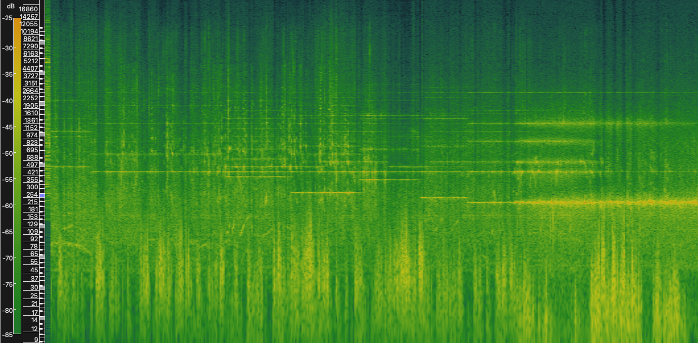
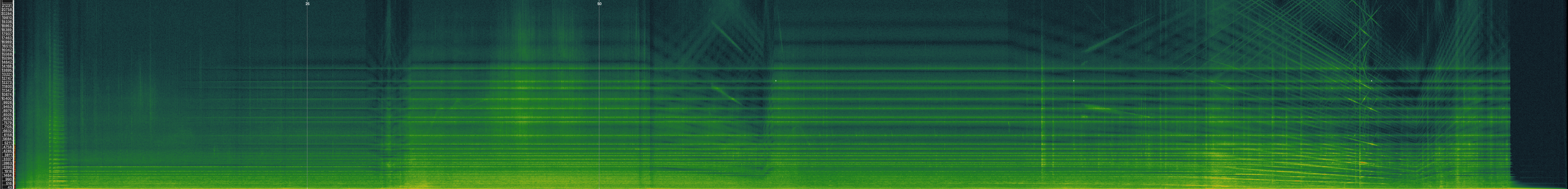
Working with Professor Paolo Girol at the Estonian Academy of Music and Theatre, I first experimented with using the bandwidth and frequency parameters to create a field of white noise which is “molded” using the filter opcodes. Here is a spectrogram image of an excerpt from the piece.


STUDY IN NOISE No. 2 - A WALK TO SCHOOL
The next opcode to be utilized was “soundin.” This opcode reads files from the computer’s disk, allowing me to start with any audio file instead of generated audio like white noise or oscillated waveforms. In later studies, this became the “diskin” opcode, which does the same task. Since that the audio was in stereo, we needed two filters to independently process both left and right channels.
Unlike study number one, this instrument only handled one frequency at a time (instead of sliding between many frequencies). But, the filters could be instanced: multiple versions of the instrument can play simultaneously, creating polyphony. It also meant that a score was needed for these instruments to play from.
This instrument also included envelope generation to give notes attack and decay, as well as pan.
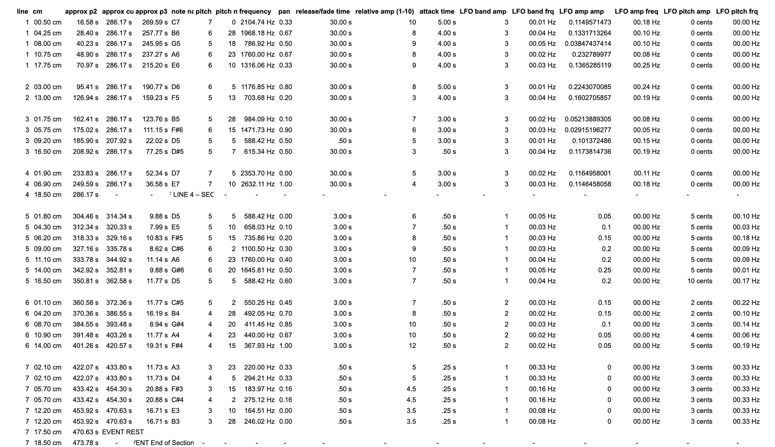
The score (<CsScore>) gives each instrument data to run an instance. Each line is like a musical note on a score– it gives information about when to start, duration, pitch, and pan. There are also bypasses to tell the instrument when to mute the field recording layer and when to mute the filtered sounds. Each “p” value connects to the code above.
The three sound files below show just the field recording (example 4), just the filtered layer (example 5), and the combination of the two (example 6).


Study in Noise No. 3 - Out my Bedroom Window

At the end of Study 3, I took advantage of this overlap to slowly build a chord which spans from lower frequencies upwards into the range where it begins overlapping with birds. In the image, the bird chirps are the short vertical lines which stretch from 3kHz to 6kHz.
Study 3, which is much longer than study 2, demonstrates the uniqueness of this synthesis method a lot better, all thanks to the birds.
In the middle of the piece, there is an elongated slow melody. When I looked at the spectrogram image, I noticed two of the notes overlapped with bird chirps between 3kHz and 4kHz, which creates a fascinating sound. Pay attention to the volume of the notes which overlap with the bird chirps.


A new way of making a score…
Instead of typing out notes and rhythms, for this piece I handwrote the composition. The number of centimeters from the beginning of the first system is translated into rhythm. To calculate frequencies, a 31 equal division of the octave tuning system was used to closely resemble an “in-tune” instrument without being exactly there. Using Google Sheets, these values are organized and calculated, and then pasted into the <CsScore> field in the code. Other values like attack and LFO modifiers for pitch and bandwidth are also entered and calculated.
Study 3 resulted in the most musical result thus far. Professor Girol stressed to me that my own satisfaction with the work was important. Out of the 3 studies I had composed, this was the only one which I felt could stand on its own as a piece of music.

Study No. 4 - At A Tram Stop
The Start of Field Recording in Tallinn
I had run out of field recordings from Ohio– but I was armed with my handy portable recorder. So, going throughout my day, I started recording things like coffee shops and the lobby in the school. One day, I recorded the sound of tram number 4 arriving at the stop– a sound I heard every day at least a couple times.
Overlaying a single chord with the filtering instruments, as the sound of the brakes get closer and the doppler effect lowers the frequency of the brakes, it slowly descended through the whole chord. Even though the amplitude of the filtered layer is not changed by the computer, it crescendos along with the noise in the field recording. This is the result.


Finalizing the Instrument’s Design
Studies in Noise 5.1 and 5.2


In composing study number 5 I returned to the ideas of manipulating the bandwidth of the filtered notes, similar to Study No. 1. To do this, I needed to play the field recording in a separate instance from the filtering process. The final code includes 2 types of instruments; the first- “instr 1” is essentially a tape machine. It calls the audio file from the drive and sends it to two global audio channels. Then, the second type (“instr 2” and “instr 3”) contains the filters which isolate frequency bands and layers them back on top. Instrument 3 is the same as instrument 2 but it is equipped with extra values which allow it to change bandwidth in the middle of a note.
Study 5.1 and 5.2 both play the same music, but using different field recordings. This example, from Study 5.1, uses a recording of the AC in my bedroom (and the sounds of my roommate on his video game through the wall). The thicker vertical line (me eating a bag of chips) starts a series of chords where top note stays the same. The bandwidth of the note expands as it is held, creating an effect of disappearing into the wind.
Study 6 - Tape Speed
The last big exploration in this set of studies, Study Number 6 focuses on a different parameter– tape speed.
Now that the instrument I had built included a separate process for the playback of field recordings, I could manipulate its parameters separate from the “music.” I wanted to find a way to speed up and slow down the tape in order to isolate specific moments in a recording.
What recording to use for this? Not the sounds of the outside world, but of another world at everyone’s fingertips: the internet.
Using an interview from NPR (which is available for download - Thank you public media!!) I employed my calculus knowledge to control the flow of time in the tape. Here is what that process looks like.


This graph shows the progression of time through both the original tape (y-axis) and the output audio (x-axis). The axes are arranged like this because when I am finished, the derivative of the black line will be my “linseg” function: the instructions I give to the computer on when to change the tape speed and how. So, what are all these lines?
Each horizontal dotted line (blue) marks a timecode along the original tape where we want to start or stop zooming ahead (i.e. “landing points”).
The vertical dotted lines represent the corresponding timecodes in the output audio where we have to start or stop manipulating the speed of the tape.
The black line shows the relationship between the original timecodes and output audio - the slope of the line is the tapespeed. It passes through the intersections of the blue and orange dotted lines.
The red line at the bottom (enlarged in the second image) shows the position of the tapespeed “knob” (referring to our imaginary tape machine). This value is never below 1 - showing that we never slow the audio down, only speed it up.
The audio example shows the first 70 seconds of resulting audio with the jumps in time.
While calculating each segment of the curve was a precise job, there is still a lot of creative choices we can make in this process. Take, for instance, the specific shape of the tape speed line. Some triangles have steep slopes, others aren’t triangles but instead trapezoids. What do these sound like? A steeper triangle translates to moving the knob forward and back faster, and trapezoids are like moving the knob halfway but then keeping it at a higher position before moving it back to normal speed. Just like playing an instrument, these shapes help us “perform” using the knob in a musical fashion.
Then, all that needed to be done was connect the shapes to their landing points using some calculus.


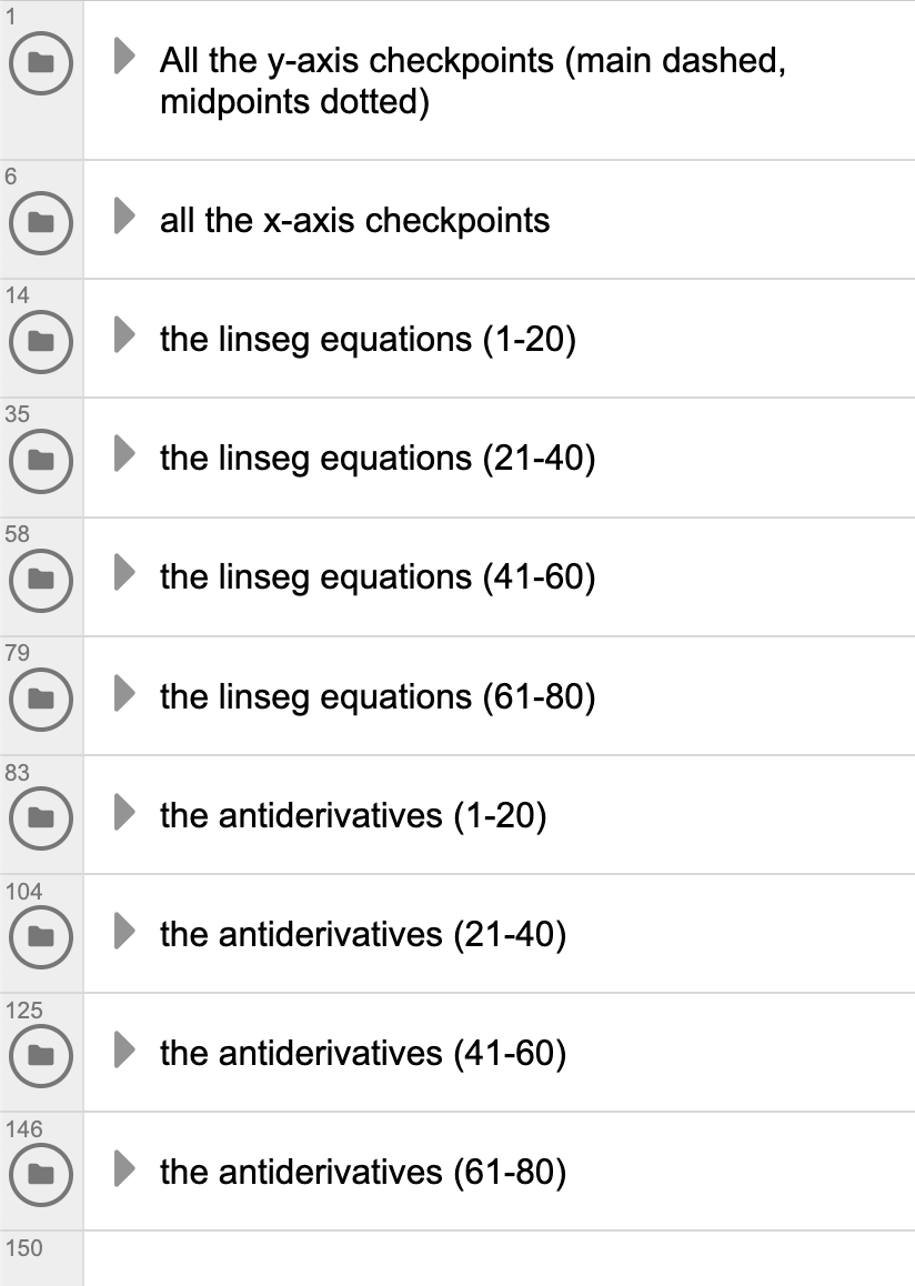
Sorted into these folders, first the timecode goals were mapped out. This was easy, just mark each point in the original tape where we want to start and stop and include the midpoint of each jump. Then, starting at (0,0), a line with a slope of 1 (for playing at normal speed) was made. The intersection was calculated and the x-position recorded. Then, when the tapespeed starts to increase, we calculate the antiderivative of the segment and keep recording x-positions as we move along, starting each new segment at the previous x-position. This way, all the lines connect in time.
Essentially, instead of guessing where the knob needed to be moved, we figure out how the jumps through the tape happen and then translate that into tapespeed value.


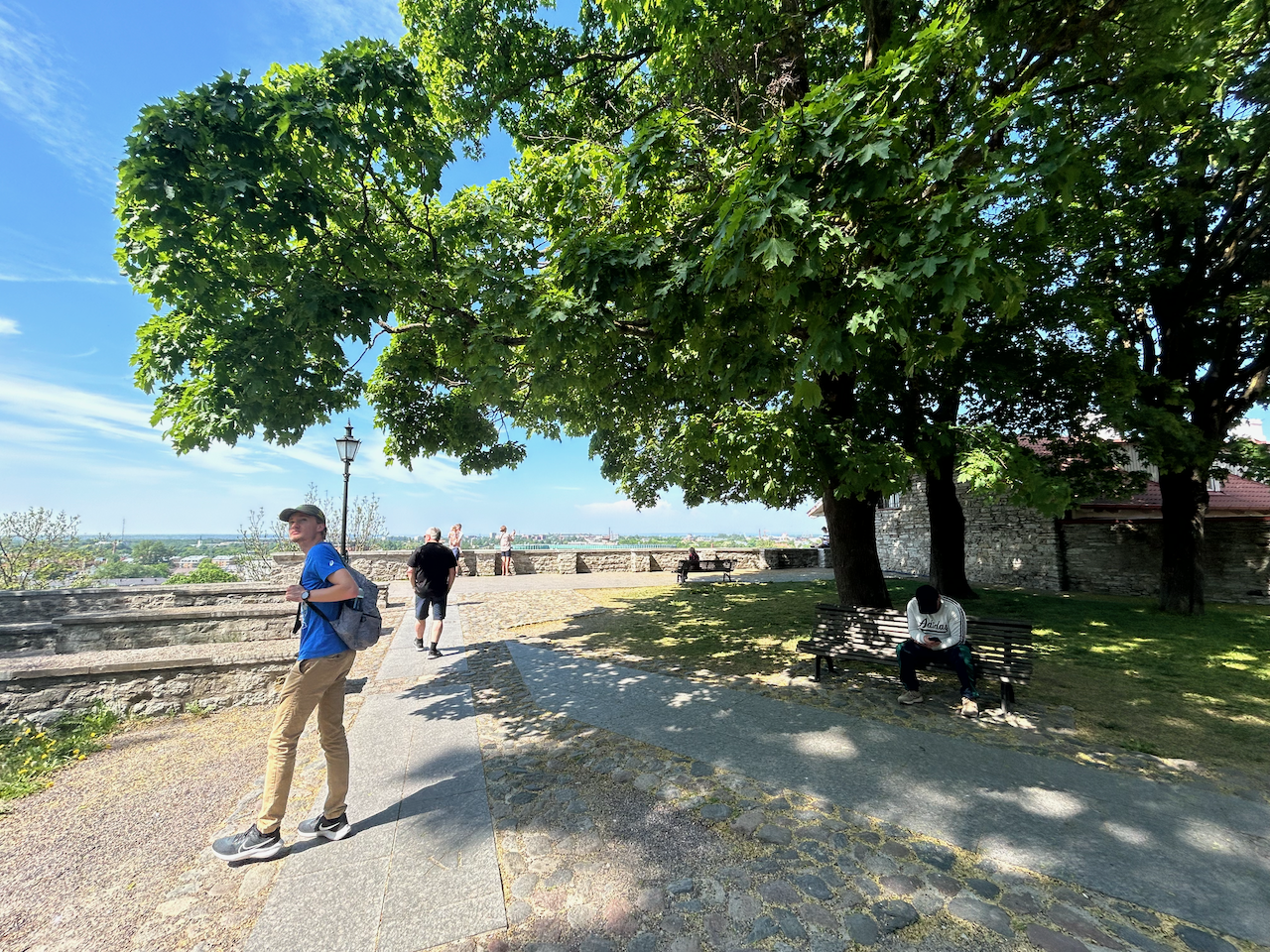
(this image is where study 7 was recorded- featuring fellow composer Aaron Reising in the blue shirt)Studies 7 and 8
The Final Studies
Studies 7 and 8
Studies 7 and 8 use techniques developed in all their preceding studies.
In Study 7, bandwidth opening techniques are paired with field recording elements and the use of speech and language found in studies 5.2 and 6.
Study 8 takes advantage of tape methods from study 6, and sourcing audio from the internet to create soundscapes not found in nature.
Premiers and Conclusions
Some of these studies were premiered at my senior recital in Columbus, OH this November. I also premiered a piece for piano and synthesizer using this same synthesis method through a MIDI controller (linked below in “other relevant works”).
Each time I brought something to a lesson Paolo asked me, “Are you satisfied with this?” This question helped me to evaluate aesthetic results with each piece of music. The final collection as it is published reflects the answers to those questions: barring studies 1 and 2, and then releasing the rest.
Political Themes & Music making outside of America
These studies are thanks to the my time at the Estonian Academy of Music and Theatre, and my study with Prof. Girol in electroacoustic composition. I would be remiss if I did not speak about how my time in Tallinn affected my perspective of being a musician from a more global perspective.
In study 7 (recorded in Tallinn) a plethora of languages make up the soundscape. This is a key aesthetic element of the music– but this is not under my control as the composer. I am grateful to those people whose voices I cannot understand as a monolingual American.
Study 8, which is directly about the Israeli/Palestinian conflict, would have been composed without the perspective from living in the same timezone where that war is happening. Granted, I was almost an entire hemisphere north, but it feels wildly different to be that close to conflicts. I feel the same about the conflict in Ukraine– especially while going to class every day with Ukrainian students.
The purpose of this page is not necessarily to show off the music… moreso the creative process behind how I explored CSound and the computer as a tool. Thank you for spending the time to read all of this, I appreciate it a lot.
If you are interested in the music, there is a button which takes you to the full album. For any other inquiries please reach out to mwrobertson02@gmail.com